Bias and Variance

The Bias-Variance trade-off
Every time you build a model, a tradeoff exists between bias and variance. One of the first things you look at are the prediction errors of the dev and test sets. You can decompose the errors into two components known as bias and variance.
Bias is an error that results from incorrect assumptions the model makes about the training data. Variance is an error that happens when the model is sensitive to small changes in the training data.
If you build a model and observe that it has a hard time predicting data it’s already seen, then your model doesn’t fit the data well. We call this high bias.
If your model is too sensitive to changes in the training data, then it will try to predict random noise rather than the intended outputs. This results in a model that will overfit your data. We call this high variance.
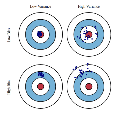
Since you want a model that minimizes bias and variance, a trade-off arises. You could have a model with a high training accuracy, but performs poorly on the dev and test sets. In this case, it’s better to sacrifice some of that training accuracy in exchange for better performance on the dev and test sets. This trade-off is perhaps more intuitively understood by the image below.

Bias-Variance decomposition
Although the bias-variance trade-off might feel experimentally familiar, it should be mathematically verified. It turns out we can decompose prediction errors into bias and variance (and an unavoidable error term).
So the data we have comes from some underlying function, $f$, mixed with some noise, $\epsilon$. Let’s represent this as $y = f + \epsilon$. Note that we assume $\epsilon$ to have a normal distribution with a mean of $0$ and variance $\sigma^2$.
The underlying function is what we’re trying to approximate with some model, $\hat{f}$. To show that the error of $\hat{f}$ in predicting $y$ (i.e. the mean squared error) is combination of bias, variance, and an irreducible error term (which is an inevitable result of the noise, $\epsilon$, in the data), we need to show that
$$ \E\big[(y - \hat{f})^2\big] = \bias\big[\hat{f}\big]^2 + \var\big[\hat{f}\big] + \sigma^2 $$
where
$$ \bias\big[\hat{f}\big] = \E\big[\hat{f} - f\big] $$
and
$$ \var\big[\hat{f}\big] = \E\Big[\hat{f}^2\Big] - \E\big[\hat{f}\big]^2 $$
So,
$$ \begin{aligned} \E\big[(y - \hat{f})^2\big] &= \E\Big[y^2 - 2y\hat{f} + \hat{f}^2\Big] \\\ &= \E\big[y^2\big] + \E\Big[\hat{f}^2\Big] - \E\big[2y\hat{f}\big] \end{aligned} $$
And since $\var[y] = \E\big[y^2\big] - \E[y]^2$ and $\var\big[\hat{f}\big] = \E\Big[\hat{f}^2\Big] - \E\big[\hat{f}\big]^2$, then with a little rearranging we have,
$$ \E\big[y^2\big] = \var[y] + \E[y]^2 $$
$$ \E\Big[\hat{f}^2\Big] = \var\big[\hat{f}\big] + \E\big[\hat{f}\big]^2 $$
So now
$$ \begin{aligned} \E\big[(y - \hat{f})^2\big] &= \var[y] + \E[y]^2 + \var\big[\hat{f}\big] + \E\big[\hat{f}\big]^2 - 2\E[y]\E[\hat{f}] \\\ &= \var[y] + \E[y]^2 + \var\big[\hat{f}\big] + \E\big[\hat{f}\big]^2 - 2f\E[\hat{f}] \\\ &= \var[y] + \var\big[\hat{f}\big] + \Big(f^2 - 2f\E[\hat{f}] + \E[\hat{f}]^2\Big) \\\ &= \var[y] + \var[\hat{f}] + (f - \E[\hat{f}])^2 \end{aligned} $$
Since $\bias[\hat{f}]^2 = \big(\E\big[\hat{f}\big] - f\big)^2 = \big(f - \E\big[\hat{f}\big]\big)^2$, we now have
$$ \E\big[(y - \hat{f})^2\big] = \var[y] + \var[\hat{f}] + \bias\big[\hat{f}\big]^2 $$
And since $\var[y] = \sigma^2$, we finally have
$$ \E\big[(y - \hat{f})^2\big] = \bias\big[\hat{f}\big]^2 + \var\big[\hat{f}\big] + \sigma^2 $$
For more justification in each of these steps, refer to the derivation procedure posted on Berkeley’s machine learning blog.
Addressing high bias and high variance
To minimize bias and variance, we need to have a game-plan for how to address high bias and high variance. In the case of high bias, we can:
- Choose a more complex model that can learn from the data.
- For neural networks, choose a better weight initialization method.
- Train the model longer.
- Choose a model that leverages boosting.
- Ensemble multiple models.
To address high variance, we have a few more options at our disposal:
- Get more data! Theoretically, variance approaches zero as the number of samples approaches infinity.
- If you can’t get more data, use data augmentation.
- Handicap your model so that it doesn’t become too complex via regularization techniques.
- Ensemble multiple models.
- Introduce some noise in the data if your data set is too clean.